Examples
Test cases are available in the PyFR-Test-Cases repository. It is important to note, however, that these examples are all relatively small 2D/3D simulations and, as such, are not suitable for scalability or performance studies.
Euler Equations
2D Euler Vortex
Proceed with the following steps to run a parallel 2D Euler vortex simulation on a structured mesh:
Navigate to the
PyFR-Test-Cases/2d-euler-vortexdirectory:cd PyFR-Test-Cases/2d-euler-vortex
Run pyfr to convert the Gmsh mesh file into a PyFR mesh file called
euler-vortex.pyfrm:pyfr import euler-vortex.msh euler-vortex.pyfrm
Run pyfr to add a partitioning to the mesh:
pyfr partition add euler-vortex.pyfrm 2
Run pyfr to solve the Euler equations on the mesh, generating a series of PyFR solution files called
euler-vortex*.pyfrs:mpiexec -n 2 pyfr -p run -b cuda euler-vortex.pyfrm euler-vortex.ini
Run pyfr on the solution file
euler-vortex-100.0.pyfrsconverting it into an unstructured VTK file calledeuler-vortex-100.0.vtu:pyfr export volume euler-vortex.pyfrm euler-vortex-100.0.pyfrs euler-vortex-100.0.vtu
Visualise the unstructured VTK file in Paraview
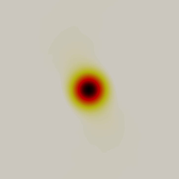
Colour map of density distribution at 100 time units.
2D Double Mach Reflection
Proceed with the following steps to run a serial 2D double Mach reflection simulation on a structured mesh:
Navigate to the
PyFR-Test-Cases/2d-double-mach-reflectiondirectory:cd PyFR-Test-Cases/2d-double-mach-reflection
Unzip the Gmsh mesh file and run pyfr to convert it into a PyFR mesh file called
double-mach-reflection.pyfrm:unxz double-mach-reflection.msh.xz pyfr import double-mach-reflection.msh double-mach-reflection.pyfrm
Run pyfr to solve the compressible Euler equations on the mesh, generating a series of PyFR solution files called
double-mach-reflection-*.pyfrs:pyfr -p run -b cuda double-mach-reflection.pyfrm double-mach-reflection.ini
Run pyfr on the solution file
double-mach-reflection-0.20.pyfrsconverting it into an unstructured VTK file calleddouble-mach-reflection-0.20.vtu:pyfr export volume double-mach-reflection.pyfrm double-mach-reflection-0.20.pyfrs double-mach-reflection-0.20.vtu
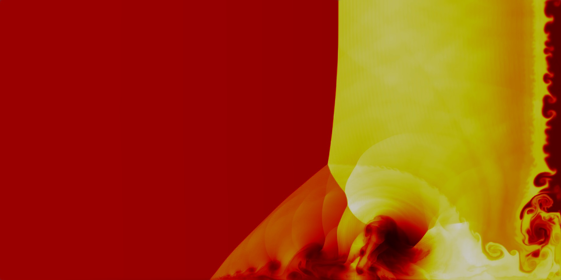
Visualise the unstructured VTK file in Paraview

Colour map of density distribution at 0.2 time units.
Navier–Stokes Equations
2D Couette Flow
Proceed with the following steps to run a serial 2D Couette flow simulation on a mixed unstructured mesh:
Navigate to the
PyFR-Test-Cases/2d-couette-flowdirectory:cd PyFR-Test-Cases/2d-couette-flow
Run pyfr to convert the Gmsh mesh file into a PyFR mesh file called
couette-flow.pyfrm:pyfr import couette-flow.msh couette-flow.pyfrm
Run pyfr to solve the Navier-Stokes equations on the mesh, generating a series of PyFR solution files called
couette-flow-*.pyfrs:pyfr -p run -b cuda couette-flow.pyfrm couette-flow.ini
Run pyfr on the solution file
couette-flow-040.pyfrsconverting it into an unstructured VTK file calledcouette-flow-040.vtu:pyfr export volume couette-flow.pyfrm couette-flow-040.pyfrs couette-flow-040.vtu
Visualise the unstructured VTK file in Paraview
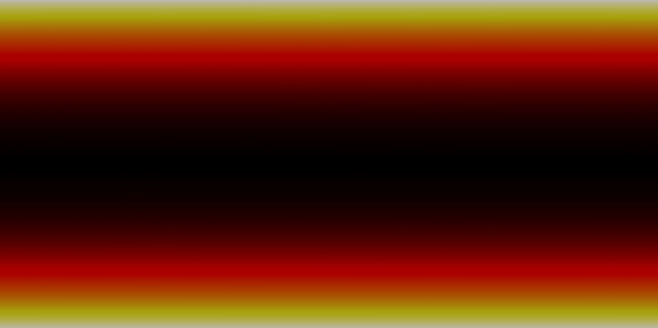
Colour map of steady-state density distribution.
2D Incompressible Cylinder Flow
Proceed with the following steps to run a serial 2D incompressible cylinder flow simulation on a mixed unstructured mesh:
Navigate to the
PyFR-Test-Cases/2d-inc-cylinderdirectory:cd PyFR-Test-Cases/2d-inc-cylinder
Run pyfr to convert the Gmsh mesh file into a PyFR mesh file called
inc-cylinder.pyfrm:pyfr import inc-cylinder.msh inc-cylinder.pyfrm
Run pyfr to solve the incompressible Navier-Stokes equations on the mesh, generating a series of PyFR solution files called
inc-cylinder-*.pyfrs:pyfr -p run -b cuda inc-cylinder.pyfrm inc-cylinder.ini
Run pyfr on the solution file
inc-cylinder-75.00.pyfrsconverting it into an unstructured VTK file calledinc-cylinder-75.00.vtu:pyfr export volume inc-cylinder.pyfrm inc-cylinder-75.00.pyfrs inc-cylinder-75.00.vtu
Visualise the unstructured VTK file in Paraview
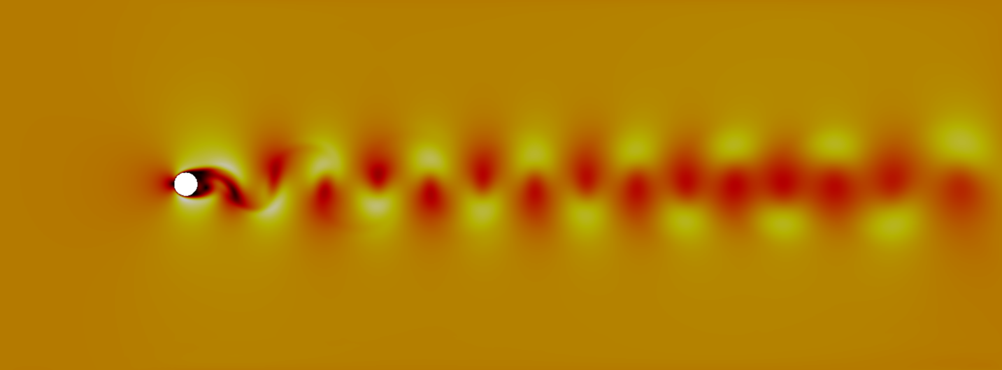
Colour map of velocity magnitude distribution at 75 time units.
2D Viscous Shock Tube
Proceed with the following steps to run a serial 2D viscous shock tube simulation on a structured mesh:
Navigate to the
PyFR-Test-Cases/2d-viscous-shock-tubedirectory:cd PyFR-Test-Cases/2d-viscous-shock-tube
Unzip the the Gmsh mesh file and run pyfr to convert it into a PyFR mesh file called
viscous-shock-tube.pyfrm:unxz viscous-shock-tube.msh.xz pyfr import viscous-shock-tube.msh viscous-shock-tube.pyfrm
Run pyfr to solve the compressible Navier-Stokes equations on the mesh, generating a series of PyFR solution files called
viscous-shock-tube-*.pyfrs:pyfr -p run -b cuda viscous-shock-tube.pyfrm viscous-shock-tube.ini
Run pyfr on the solution file
viscous-shock-tube-1.00.pyfrsconverting it into an unstructured VTK file calledviscous-shock-tube-1.00.vtu:pyfr export volume viscous-shock-tube.pyfrm viscous-shock-tube-1.00.pyfrs viscous-shock-tube-1.00.vtu
Visualise the unstructured VTK file in Paraview
Colour map of density distribution at 1 time unit.
3D Triangular Aerofoil
Proceed with the following steps to run a serial 3D triangular aerofoil simulation with inflow turbulence:
Navigate to the
PyFR-Test-Cases/3d-triangular-aerofoildirectory:cd PyFR-Test-Cases/3d-triangular-aerofoil
Unzip the Gmsh mesh file and run pyfr to convert it into a PyFR mesh file called
triangular-aerofoil.pyfrm:unxz triangular-aerofoil.msh.xz pyfr import triangular-aerofoil.msh triangular-aerofoil.pyfrm
Run pyfr to solve the Navier-Stokes equations on the mesh, generating a series of PyFR solution files called
triangular-aerofoil-*.pyfrs:pyfr -p run -b cuda triangular-aerofoil.pyfrm triangular-aerofoil.ini
Run pyfr on the solution file
triangular-aerofoil-5.00.pyfrsconverting it into an unstructured VTK file calledtriangular-aerofoil-5.00.vtu:pyfr export volume triangular-aerofoil.pyfrm triangular-aerofoil-5.00.pyfrs triangular-aerofoil-5.00.vtu
Visualise the unstructured VTK file in Paraview
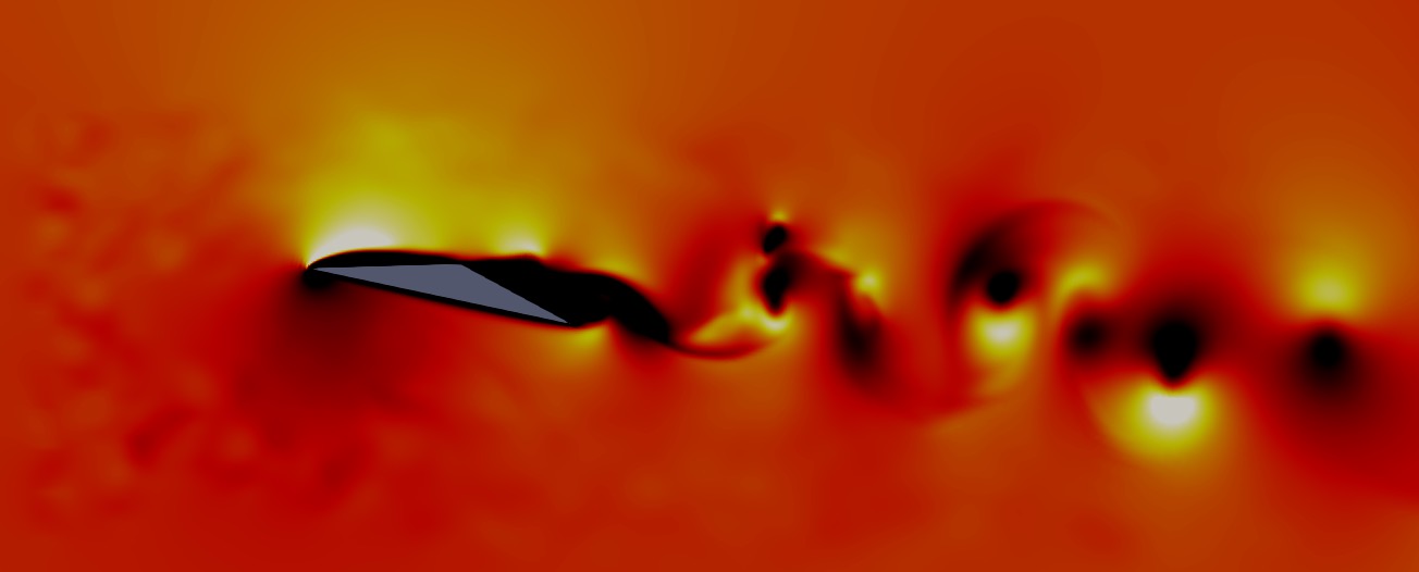
Colour map of velocity magnitude distribution at 5 time units.
If you have installed Ascent you can run the same case with the [soln-plugin-ascent] plugin activated, which will produce a series of .png images that can then be merged into an animation using a utility such as ffmpeg:
pyfr -p run -b cuda triangular-aerofoil.pyfrm triangular-aerofoil-ascent.ini
3D Taylor-Green
Proceed with the following steps to run a serial 3D Taylor-Green simulation:
Navigate to the
PyFR-Test-Cases/3d-taylor-greendirectory:cd PyFR-Test-Cases/3d-taylor-green
Unzip the Gmsh mesh file and run pyfr to convert it into a PyFR mesh file called
taylor-green.pyfrm:unxz taylor-green.msh.xz pyfr import taylor-green.msh taylor-green.pyfrm
Run pyfr to solve the Navier-Stokes equations on the mesh, generating a series of PyFR solution files called
taylor-green-*.pyfrs:pyfr -p run -b cuda taylor-green.pyfrm taylor-green.ini
Run pyfr on the solution file
taylor-green-5.00.pyfrsconverting it into an unstructured VTK file calledtaylor-green-5.00.vtu:pyfr export volume taylor-green.pyfrm taylor-green-5.00.pyfrs taylor-green-5.00.vtu
Visualise the unstructured VTK file in Paraview
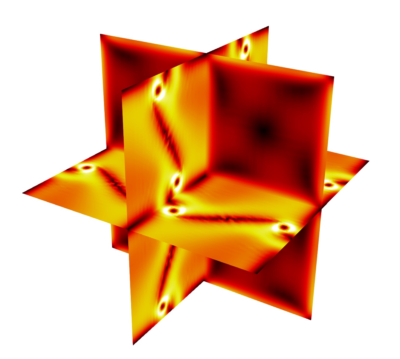
Colour map of velocity magnitude distribution at 5 time units.
If you have installed Ascent you can run the same case with the [soln-plugin-ascent] plugin activated, which will produce a series of .png images that can then be merged into an animation using a utility such as ffmpeg:
pyfr -p run -b cuda taylor-green.pyfrm taylor-green-ascent.ini